R語言文字探勘好好玩 - Ch2_採 Tidy 資料做情感分析 (2)

前面一章是解釋說明什麼是 怎麼運用詞典來看出小說的情緒分析,本篇就延續下去介紹詞雲的圖形的視覺化,在本篇的介紹大綱裡面包含如下:

學習內容大綱

  1. 最常見的正面詞和負面詞
  2. 詞雲

最常見的正面詞和負面詞

同時使用包含情感與詞的分析,可以對情感知道貢獻的詞次數。使用 word, sentiment 計算一下 count 次數,可以看看哪一個詞貢獻多大。

1
2
3
4
5
6
bing_word_counts <- tidy_books %>%
inner_join(get_sentiments("bing")) %>%
count(word, sentiment, sort = TRUE) %>%
ungroup()

bing_word_counts

結果如下:

1
2
3
4
5
6
7
8
9
10
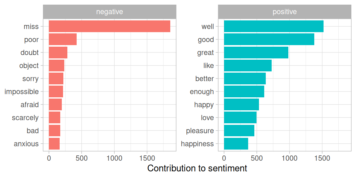
# A tibble: 2,585 x 3
word sentiment n
<chr> <chr> <int>
1 miss negative 1855
2 well positive 1523
3 good positive 1380
4 great positive 981
5 like positive 725
6 better positive 639
7 enough positive 613

接著我們可以透過 ggplot2 呈現結果

1
2
3
4
5
6
7
8
9
10
11
bing_word_counts %>%
group_by(sentiment) %>%
top_n(10) %>%
ungroup() %>%
mutate(word = reorder(word, n)) %>%
ggplot(aes(word, n, fill = sentiment)) +
geom_col(show.legend = FALSE) +
facet_wrap(~sentiment, scales = "free_y") +
labs(y = "Contribution to sentiment",
x = NULL) +
coord_flip()

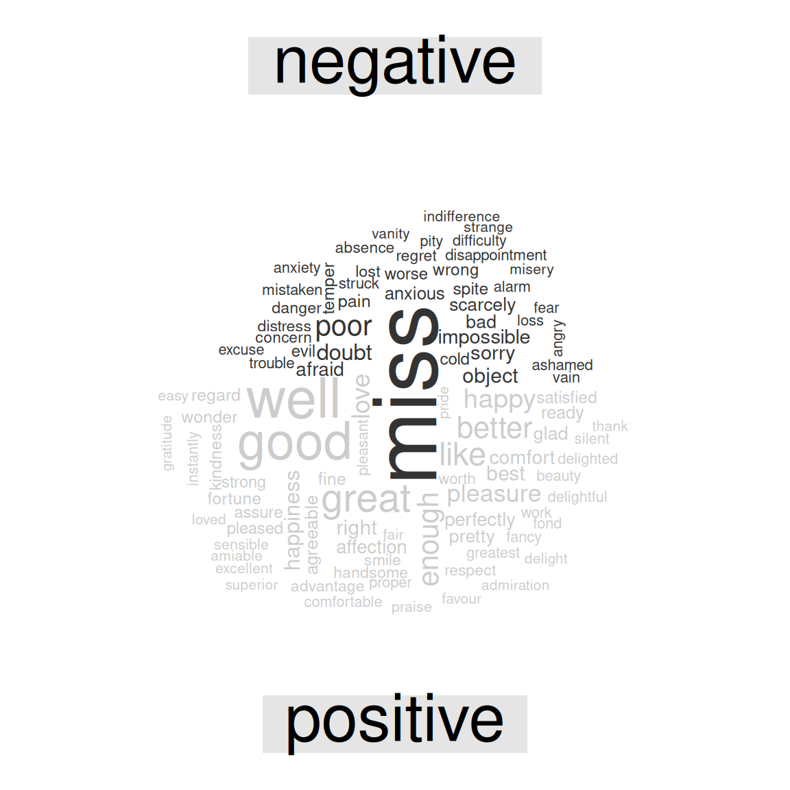
這邊值得一提的是,在負面情緒裡面的第一個 miss 反而是被當作為負面詞,而這不太符合目的。可以利用 bind_rows() 把這樣的詞加進自定義停用詞裡,我們定義這個欄位為 lexicon

1
2
3
4
custom_stop_words <- bind_rows(data_frame(word = c("miss", "hung", "well", "master"),
lexicon = c("custom")),
stop_words)
custom_stop_words

結果如下:

1
2
3
4
5
6
7
8
9
10
# A tibble: 1,153 x 2
word lexicon
<chr> <chr>
1 miss custom
2 hung custom
3 well custom
4 master custom
5 a SMART
6 a's SMART
7 able SMART

詞雲

在前幾節的說明,都有用 ggplot2 來做視覺化的繪圖,在這節裡,使用 wordcloud 套件來看詞頻的狀況。

1
2
3
4
5
6
library(wordcloud)

tidy_books %>%
anti_join(stop_words) %>%
count(word) %>%
with(wordcloud(word, n, max.words = 100))

結果如下:

由於我們使用的 wordcloud 套件,裡頭包含了 comparison.cloud() 部分,可以用 reshape2acast() 把數據轉變成矩陣,找到最常見的正面與負面詞,字越大的話,代表貢獻度也越大

1
2
3
4
5
6
7
8
library(reshape2)

tidy_books %>%
inner_join(get_sentiments("bing")) %>%
count(word, sentiment, sort = TRUE) %>%
acast(word ~ sentiment, value.var = "n", fill = 0) %>%
comparison.cloud(colors = c("gray20", "gray80"),
max.words = 100)

結果如下:

參考

  1. Text Mining with R